Rethinking Decision Transformer via Hierarchical Reinforcement Learning

Abstract

$Decision Transformer (DT) is an innovative algorithm leveraging recent advances of the transformer architecture in reinforcement learning (RL). However, a notable limitation of DT is its reliance on recalling trajectories from datasets, losing the capability to seamlessly Stitch sub-optimal trajectories together. In this work we introduce a general sequence modeling framework for studying sequential decision making through the lens of Hierarchical RL. At the time of making decisions, a high-level policy first proposes an ideal prompt for the current state, a low-level policy subsequently generates an action conditioned on the given prompt. We show DT emerges as a special case of this framework with certain choices of high-level and low-level policies, and discuss the potential failure of these choices. Inspired by these observations, we study how to jointly optimize the high-level and low-level policies to enable the stitching ability, which further leads to the development of new offline RL algorithms. Our empirical results clearly show that the proposed algorithms significantly surpass DT on several control and navigation benchmarks. We hope our contributions can inspire the integration of transformer architectures within the field of RL.

Autotuned Decision Transformer (ADT)

Definition of ADT

Our algorithm is derived by considering a general framework that bridges transformer-based decision models with hierarchical reinforcement learning (HRL). In particular, we use the following hierarchical representation of policy

$ \pi(a | s) = \int_{\mathcal{P}} \pi^{h}(p | s) \cdot \pi^{l} (a | s, p) dp\, , $ where $\mathcal{P}$ is a set of prompts. To make a decision, the high-level policy $\pi^h$ first generates a prompt $p\in \mathcal{P}$, instructed by which the low-level policy $\pi^l$ returns an action conditioned on $p$.

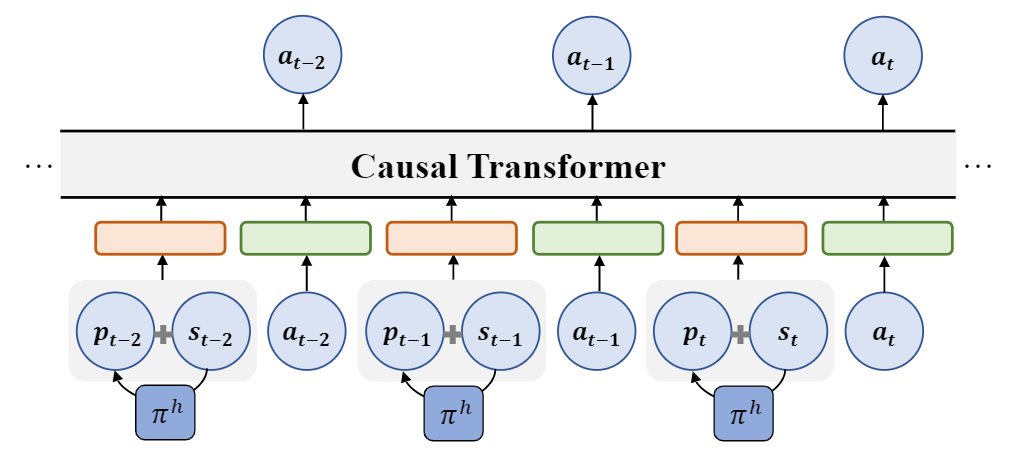
ADT jointly optimizes the hierarchical policies to overcomes the limitations of DT. An illustration of ADT architecture is provided in the figure above. Similar to DT, ADT applies a transformer model for the low-level policy, it considers the following trajectory representation, $ \tau=\left(p_0, s_0, a_0, p_1, s_1, a_1, \ldots, p_T, s_T, a_T\right) $ Here $p_i$ is the prompt generated by the high-level policy $p_i \sim \pi^h(\cdot | s_i)$, replacing the return-to-go prompt used by DT. That is, for each trajectory in the offline dataset, we relabel it by adding a prompt generated by the high-level policies for each transition. Armed with this general hierarchical decision framework, we propose two algorithms that apply different high-level prompting generation strategy while sharing a unified low-level policy optimization framework. We learn a high-level policy $\pi_\omega\approx \pi^h$ with parameters $\phi$, and a low-level polic y $\pi_\theta \approx \pi^l$ with parameters $\theta$.

Value-prompted Autotuned Decision Transformer (V-ADT)

Our first algorithm, \emph{Value-promped Autotuned Decision Transformer (V-ADT)}, uses scalar values as prompts. But unlike DT, it applies a more principled design of value prompts instead of return-to-go.
V-ADT aims to answer two questions: what is the maximum achievable value starting from a state $s$, and what action should be taken to achieve such a value?
The optimal value of this empirical MDP presented by the offline dataset is $ V_{\mathcal{D}}^*(s)=\max _{a: \pi_{\mathcal{D}}(a \mid s)>0} r(s, a)+\gamma \mathbb{E}_{s^{\prime} \sim P_{\mathcal{D}}(\cdot \mid s, a)}. $

Let $Q_{\mathcal{D}}^*(s, a)$ be the corresponding state-action value. $V_{\mathcal{D}}^*$ is known as the in-sample optimal value in offline RL. We now describe how V-ADT jointly optimizes high and low level policies to facilitate stitching.

High-Level policy

High-Level policy V-ADT adopts a deterministic policy $\pi_\omega: \mathcal{S} \rightarrow \mathbb{R}$, which predicts the in-sample optimal value $\pi _\omega \approx V_{\mathcal{D}}^*$. Since we already have an approximated in-sample optimal value $V_\phi$, we let $\pi_\omega=V_\phi$. This high-level policy offers two key advantages. First, this approach efficiently facilitates information backpropagation towards earlier states on a trajectory, addressing a major limitation of DT. This is achieved by using $V_{\mathcal{D}}^*$ as the value prompt, ensuring that we have precise knowledge of the maximum achievable return for any state. Making predictions conditioned on $R^*(s)$ is not enough for policy optimization, since $R^*(s)=\max _{\tau \in \mathcal{T}(s)} R(\tau)$ only gives a lower bound on $V_{\mathcal{D}}^*(s)$ and thus would be a weaker guidance (see Section 3.1 for detailed discussions). Second, the definition of $V_{\mathcal{D}}^*$ exclusively focuses on the optimal value derived from observed data and thus avoids out-of-distribution returns. This prevents the low-level policy from making decisions conditioned on prompts that require extrapolation.

Low-Level policy

Low-Level policy Directly training the model to predict the trajectory, as done in DT, is not suitable for our approach. This is because the action $a_t$ observed in the data may not necessarily correspond to the action at state $s_t$ that leads to the return $V_{\mathcal{D}}^*\left(s_t\right)$. However, the probability of selecting $a_t$ should be proportional to the value of this action. Thus, we use advantage-weighted regression to learn the low-level policy: given trajectory data, the objective is defined as $ \mathcal{L}(\theta)=-\sum_{t=0}^T \exp \left(\frac{Q_\psi\left(s_t, a_t\right)-V_\phi\left(s_t\right)}{\alpha}\right) \log \pi_\theta\left(a_t \mid s_t, \pi_\omega\left(s_t\right)\right), $ where $\alpha>0$ is a hyper-parameter. The low-level policy takes the output of high-level policy as input. This guarantees no discrepancy between train and test value prompt used by the policies. We note that the only difference of this compared to the standard maximum log-likelihood objective for sequence modeling is to apply a weighting for each transition. One can easily implement this with trajectory data for a transformer. In practice we also observe that the tokenization scheme when processing the trajectory data affects the performance of ADT. Instead of treating the prompt $p_t$ as a single token as in DT, we find it is beneficial to concatenate $p_t$ and $s_t$ together and tokenize the concatenated vector.

Goal-prompted Autotuned Decision Transformer (G-ADT)

In HRL, the high-level policy often considers a latent action space. Typical choices of latent actions includes sub-goal, skills, and options. We consider goal-reaching problem as an example and use subgoals as latent actions, which leads to our second algorithm, Goal-promped Autotuned Decision Transformer (G-ADT). Let $\mathcal{G}$ be the goal space ${ }^3$. The goal-conditioned reward function $r(s, a, g)$ provides the reward of taking action $a$ at state $s$ for reaching the goal $g \in \mathcal{G}$. Let $V(s, g)$ be the universal value function defined by the goal-conditioned rewards. Similarly, we define $V_{\mathcal{D}}^*(s, g)$ and $Q_{\mathcal{D}}^*(s, a, g)$ the in-sample optimal universal value function. We also train $V_\phi \approx V_{\mathcal{D}}^*$ and $Q_\psi \approx Q_{\mathcal{D}}^*$ to approximate the universal value functions. We now describe how G-ADT jointly optimizes the policies.

High-Level policy

G-ADT considers $\mathcal{P}=\mathcal{G}$ and uses a high-level policy $\pi_\omega: \mathcal{S} \rightarrow \mathcal{G}$. To find a shorter path, the high-level policy $\pi_\omega$ generates a sequence of sub-goals $g_t=\pi_\omega\left(s_t\right)$ that guides the learner step-by-step towards the final goal. We use a sub-goal that lies in $k$-steps further from the current state, where $k$ is a hyper-parameter of the algorithm tuned for each domain (Badrinath et al., 2023; Park et al., 2023). In particular, given trajectory data (4), the high-level policy learns the optimal $k$-steps jump using the recently proposed Hierarchical Implicit Q-learning (HIQL) algorithms: $ \begin{aligned} & \mathcal{L}(\phi)=-\sum_{t=0}^T \exp \left(\frac{\mathcal{A}_{\text {high }}}{\alpha}\right) \log \pi_\omega\left(s_{t+k} \mid s_t, g\right)
& \mathcal{A}_{\text {high }}=\sum_{t^{\prime}=t}^{k-1} \gamma^{t^{\prime}-t} r\left(s_{t^{\prime}}, a_{t^{\prime}}, g\right)+\gamma^k V_\phi\left(s_{t+k}, g\right)-V_\phi\left(s_t, g\right) \end{aligned} $

Low-Level policy

The low-level policy in G-ADT learns to reach the sub-goal generated by the high-level policy. GADT shares the same low-level policy objective as V-ADT. Given trajectory data, it considers the following $ \mathcal{L}(\theta)=-\sum_{t=0}^T \exp \left(\frac{\mathcal{A}_{\text {low }}}{\alpha}\right) \cdot \log \pi_\theta\left(a_t \mid s_t, \pi_\omega\left(s_t\right)\right), $ where $\mathcal{A}_{\text {low }}=Q_\psi\left(s_t, a_t, \pi_\omega\left(s_t\right)\right)-V_\phi\left(s_t, \pi_\omega\left(s_t\right)\right)$. Note that this is exactly the same as that in V-ADT except that the advantages $\mathcal{A_\text{low}}$ are computed by universal value functions. G-ADT also applies the same tokenization method as V-ADT by first concatenating $\pi_\omega(s_t)$ and $s_t$ together. This concludes the description of the G-ADT algorithm.

Experiments

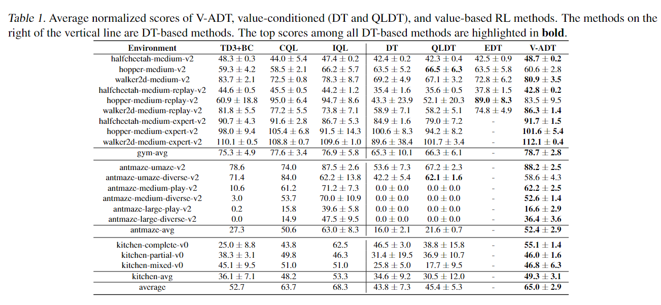
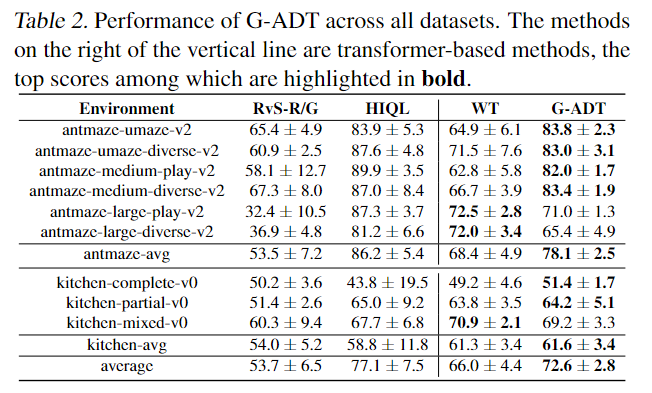
Table 1 and 2 present the performance of two variations of ADT evaluated on offline datasets. ADT significantly outperforms prior transformer-based decision making algorithms. Compared to DT and QLDT, two transformer-based algorithms for decision making, V-ADT exhibits significant superiority especially on AntMaze and Kitchen which require the stitching ability to success. Meanwhile, Table 2 shows that G-ADT significantly outperforms WT, an algorithm that uses sub-goal as prompt for a transformer policy. We note that ADT enjoys comparable performance with state-of-the-art offline RL methods. For example, V-ADT outperforms all offline RL baselines in Mujoco problems. In AntMaze and Kitchen, V-ADT matches the performance of IQL, and significantly outperforms TD3+BC and CQL. Table 2 concludes with similar findings for G-ADT.